Markov Chains are integral component of Markov Chain Monte Carlo (MCMC) techniques. Under MCMC Markov Chain is used to sample from some target distribution. This post tries to develop basic intuition about what Markov Chain is and how we can use it to sample from a distribution.

In a layman terms we can define Markov Chain as a collection of random variables having the property that, given the present, the future is conditionally independent of the past. This might may not make sense to you right now but this will be the core of the discussion when we discuss about MCMC algorithms.

Lets us now take a formal (mathematical) look at the definition of Markov Chain and some of its properties. A Markov Chain is a stochastic process that undergoes transition from one state to another on a given set of states called state space of Markov Chain.

I used a term stochastic process which is a random process that evolves with time. We can perceive it as probabilistic counterpart of a deterministic process where instead of evolving in a one way (deterministic) process can have multiple directions in which it can evolve or it has some kind of indeterminacy to its future. One example of a stochastic process is Brownian Motion.

A Markov is characterised by following three elements:

• A state space $Val(X)$, which is a set of values (state $x$) chain is allowed to take.

• A transition model $T$, which specifies for each pair of state $x$, $x'$ the probability $T (x \rightarrow x')$ of going from $x$ to $x'$.

• An initial state distribution $P^{(0)}(X^{(0)} = x)$, $\forall x \in Val(X)$, which defines the probability of being in any one of the possible states at the initial iteration t = 0.

We can define distribution over subsequent time $P^{(1)}(X^{(1)})$, $P^{(2)}(X^{(2)})$, $P^{(3)}(X^{(3)})$, $\cdots$ using chain dynamics as

$P^{(t+1)}(X^{(t+1)} = x)$ = $\sum_{x' \in Val(x)}P^{(t)}(X^{(t)} = x')T(x' \rightarrow x)$

I earlier described a porperty of Markov chain which was

Given the present, the future is conditionally independent of the past

This property is called as Markov Property or memoryless property of Markov chain, which is mathematically described as:

There are other two properties of interest which we can usually find in most of the real life application of Markov Chains:

• Stationarity : Let sequence $X_1, X_2, X_3, X_4, \cdots$ of some random elements of some set be a stochastic process, then a stochastic process is stationary if for every positive integer k the distribution of the k-tuple $(X_{n+1}, X_{n+2},\cdots,X_{n+k})$ does not depend on ‘n’. Thus a Markov Chain is stationary if it is stationary stochastic process. This stationarity property in Markov Chains implies stationary transition probabilities which in turn gives rise to equilibrium distribution. It is not necessary that all Markov Chains have equilibrium distribution but all Markov Chains used in MCMC do.

• Reversibility: A Markov Chain is reversible if the probability of transition $P^{(t)}(X^{(t)}) \rightarrow P^{(t+1)}(X^{(t+1)})$ is same as the probability of reverse transition $P^{(t+1)}(X^{(t+1)}) \rightarrow P^{(t)}(X^{(t)})$. Reversibility in Markov Chain implies stationarity.

Finite State Space Markov Chain

If the state space of Markov Chain takes on a finite number of distinct values, the transition operator can be defined using a square matrix $T$

The entry $p_{ij}$ represents transition probability of moving from state $x_i$ to state $x_j$.

Lets first use an example Markov chain and understand these terms using that. I’ll use a Markov chain to simulate Gambler’s Ruin problem. In this problem suppose that there are two players $P_1$ and $P_2$ playing poker. Initially both of them had $\$2$ with them. In each round winner gets a dollar and loser loses one and game will continue till any one of them loses his all money. Consider that probability of winning for $P_1$ is $0.49$. Our task is to estimate probability of winning the complete game for player $P_1$. Here is how our Markov chain will look like:

The state space of Markov Chain is $\{0, 1, 2, 3, 4\}$ As state space is finite, we can write the transition model in form of a matrix as

transition = [[1, 0, 0, 0, 0],
              [0.51, 0, 0.49, 0, 0],
              [0, 0.51, 0, 0.49, 0],
              [0, 0, 0.51, 0, 0.49],
              [0, 0, 0, 0, 1]]

The initial money with $P_1$ is $2$, so we can consider start state as vector start = [0, 0, 1, 0, 0]. Now with these characterisation we will simulate our Markov Chain and try to reach stationary distribution, which will give us probability of winning.

import numpy as np
import matplotlib.pyplot as plt
iterations = 30  # Simulate chain for 30 iterations
initial_state = np.array([[0, 0, 1, 0, 0]])
transition_model = np.array([[1, 0, 0, 0, 0], [0.51, 0, 0.49, 0, 0], [0, 0.51, 0, 0.49, 0],
                             [0, 0, 0.51, 0, 0.49], [0, 0, 0, 0, 1]])
transitions = np.zeros((iterations, 5))
transitions[0] = initial_state
for i in range(1, iterations):
    transitions[i] = np.dot(transitions[i-1], transition_model)
labels = [0, 0, 0, 0, 0, 0]
plt.figure()
plt.hold(True)
plt.plot(transitions)
labels[0], = plt.plot(range(iterations), transitions[:,0], color='r')
labels[1], = plt.plot(range(iterations), transitions[:,1], color='b')
labels[2], = plt.plot(range(iterations), transitions[:,2], color='g')
labels[3], = plt.plot(range(iterations), transitions[:,3], color='m')
labels[4], = plt.plot(range(iterations), transitions[:,4], color='c')
labels[5], = plt.plot([20, 20], [0, 1.2], color='k', linestyle='dashed')
plt.legend(labels, ['money=0','money=1','money=2','money=3', 'money=4', 'burn-in'])
plt.hold(False)
#plt.show()
print("Probability of winning the complete game for P1 is", transitions[iterations - 1][4])

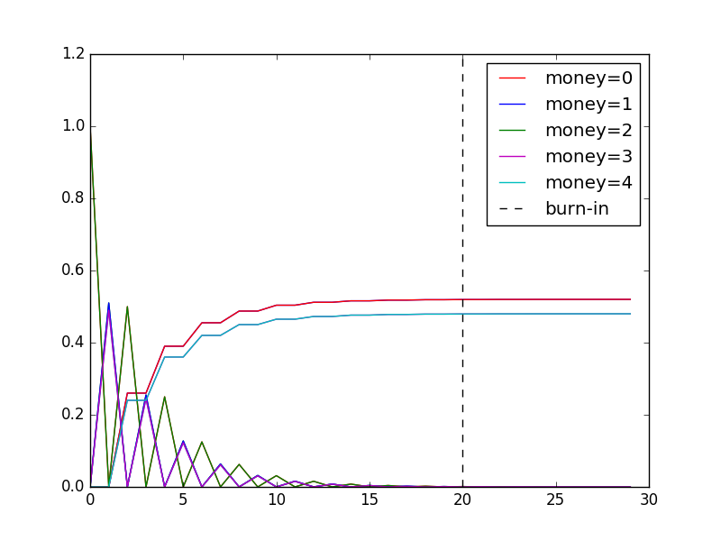
The output of above code sample is: Probability of winning the complete game for P1 is 0.479978863078, which is a good approximation of original result 0.48(see the link, for calculation of exact result). In Trace plot of Markov chain one can see that in starting there were fluctuations but after some-time chain reached an equilibrium/stationary distribution as probabilities are not changing much in subsequent iterations. Mathematically a distribution $\pi(X=x)$ is a stationary distribution if it satisfies following property:

Using the above property we can see that our chain has approximately reached stationary distribution as following condition returns True.

np.allclose(transitions[-1], np.dot(transitions[-1], transition_model), atol=1e-04)

The initial period of about 20 iterations(here) is called burn-in period of Markov Chain( see the dotted line in plot ) and is defined as the number of iterations it takes the chain to move from initial conditions to stationary distribution. I find Burn-in period to be a misleading term so I’ll call it Warm-up period. The Burn-in term was used by early authors of MCMC who were from physics background and has been used since then :/ .

One interesting thing about stationary Markov chains is that it is not necessary to sequentially iterate to predict future state. One can predict future state by raising the transition operator to the N-th power, where N is the iteration a which we want to predict, and then multiplying it by the initial distribution. For example if we wanted to predict probabilities after 24 iteration we could simply have done:

Lets look at a more interesting application of stationary Markov chain. Here we will create our own naive page ranking algorithm using a Markov Chain. For computing transition probabilities from page $i$ to $j$ (for all pairs of $i$ , $j$) we use a configuration parameter $\alpha$ and two factors which are dependent on the number of pages that links to $i$ and whether the page $j$ has link to page $i$. Here is a python code for the same:

import matplotlib.pyplot as plt
import numpy as np

alpha = 0.77  # Configuration parameter
iterations = 20
num_world_wide_web_pages = 4.0
# Consider world wide web has 4 web pages only
# Following is mapping between number of links to page
links_to_page = {0: 3, 1: 3, 2: 1, 3: 2}

# Returns transition probability of x -> y
def get_transition_probabilities(links_to_page, linked):
    global alpha
    global num_world_wide_web_pages
    constant_val = (1.0 - alpha)/num_world_wide_web_pages
    if linked is True:
        return (alpha/links_to_page) + constant_val
    else:
        return constant_val

transition_probs = np.zeros((4,4))
# Page 1 is not linked to itself
transition_probs[0][0] = get_transition_probabilities(links_to_page[0], False)
# Page 1 is linked to every other page
for i in range(1,4):
    transition_probs[0][i] = get_transition_probabilities(links_to_page[0], True)
# Page 2 is not linked to itself
transition_probs[1][1] = get_transition_probabilities(links_to_page[1], False)
# Page 2 is linked to every other page
for i in [0, 2, 3]:
    transition_probs[1][i] = get_transition_probabilities(links_to_page[1], True)
# Page 3 is only linked to page 4
transition_probs[2][3] = get_transition_probabilities(links_to_page[2], True)
# Page 3 is not linked to every other page except 4
for i in range(3):
    transition_probs[2][i] = get_transition_probabilities(links_to_page[2], False)
# Page 4 is linked to 1 and 3 and is not linked to 2 and itself
for i in range(4):
    transition_probs[3][i] = get_transition_probabilities(links_to_page[3], not i%2)

transitions = np.zeros((iterations, 4))
transitions[0] = np.array([1, 0, 0, 0])  # Starting markov chain from page 1, initial distribution

for i in range(1, iterations):
    transitions[i] = np.dot(transitions[i-1], transition_probs)

labels = [0, 0, 0, 0, 0]
plt.figure()
plt.hold(True)
labels[0], = plt.plot(range(iterations), transitions[:,0], color='b')
labels[1], = plt.plot(range(iterations), transitions[:,1], color='r')
labels[2], = plt.plot(range(iterations), transitions[:,2], color='g')
labels[3], = plt.plot(range(iterations), transitions[:,3], color='k')
labels[4], = plt.plot([10, 10], [0, 1], color='y', linestyle='dashed')
plt.legend(labels, ['page 1', 'page 2', 'page 3', 'page 4', 'burn-in'])
plt.hold(False)
plt.show()

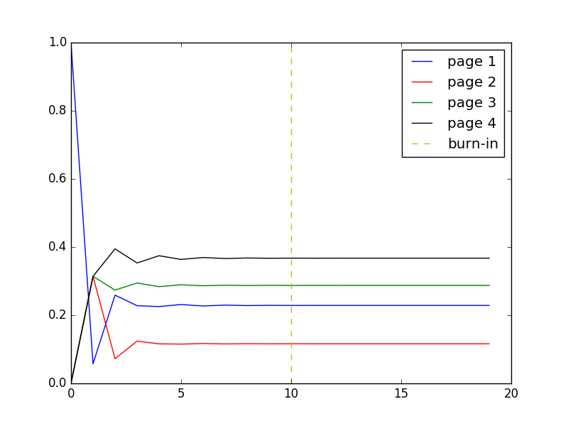
Our algorithm will rank pages in order Page 4, Page 3, Page 1, Page 2 :o .

Continuous State-Space Markov Chains

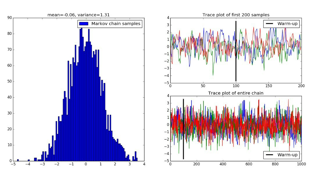
A Markov chain can also have continuous state space that exist in real numbers $x \in R^N$. In this we cannot represent transition operator as a matrix , but instead we represent it as a continuous function on the real numbers. Like Finite state-space Markov chains continuous state-space Markov chains also have a warm-up period and a stationary distribution but here stationary distribution is also over continuous set of variables.

Lets look at example on how to use a continuous state space Markov chain to sample from continuous distribution. Here our transition operator will be normal distribution with mean as half of the distance between zero and previous state and unit variance. We will throw away certain amount of states generated in start as they will be in warm-up period , the subsequent states that our chain reaches in stationary distribution will be our samples. Also we can run multiple chains simultaneously to draw samples more densely.

import numpy as np
import matplotlib.pyplot as plt

np.random.seed(71717)
warm_up = 100
n_chains = 3

transition_function = lambda x, n_chains: np.random.normal(0.5*x, 1, n_chains)
n_iterations = 1000
x = np.zeros((n_iterations, n_chains))
x[0] = np.random.randn(n_chains)

for it in range(1, n_iterations):
    x[it] = transition_function(x[it-1], n_chains)

plt.figure()
plt.subplot(222)
plt.plot(x[0:200])
plt.hold(True)
minn = min(x.flatten())
maxx = max(x.flatten())
l = plt.plot([warm_up, warm_up],[minn, maxx], color='k', lw=3)
plt.legend(l, ['Warm-up'])
plt.title('Trace plot of first 200 samples')
plt.hold(False)
plt.subplot(224)
plt.plot(x)
plt.hold(True)
l = plt.plot([warm_up, warm_up],[minn, maxx], color='k', lw=3)
plt.legend(l, ['Warm-up'], loc='lower right')
plt.title("Trace plot of entire chain")
plt.hold(False)
samples = x[warm_up+1:,:].flatten()
plt.subplot(121)
plt.hist(samples, 100)
plt.legend(["Markov chain samples"])
mu = round(np.mean(samples), 2)
var = round(np.var(samples), 2)
plt.title("mean={}, variance={}".format(mu, var))
plt.show()

Ending Note

In the above examples we deduced the stationary distribution based on observation and gut feeling :P . However, in order to use Markov chains to sample from a specific target distribution, we have to design the transition operator such that the resulting chain reaches a stationary distribution that matches the target distribution. This is where MCMC methods come to rescue.